G3→G6 Value-Added (Bayesian)
A two-stage Bayesian approach. Stage 1: estimate each school's G3 quality from three years of Grade 3 binomial data (2022–23 through 2024–25). Stage 2: fit a G6 binomial GLMM with the G3 school quality estimate as a covariate — the residual G6 school random effect is the value-added component.
Model structure
| Stage 1 | Stage 2 | |
|---|---|---|
| Outcome | G3 L3/4 successes | trials | G6 L3/4 successes | trials |
| Data | Long G3, 2023–2025, 3 subjects | Long G6, 2023–2025, 3 subjects |
| Fixed effects | Year×subject cells | Year×subject cells, G3 school RE (me-corrected) |
| Random effects | School | School (= VA), School×year |
| School RE output | G3 quality estimate → Stage 2 input | Value-added estimate |
The G3 quality estimates come from the Stage 1 production M2 model described on the Bayesian Multilevel page — M2 (year×subject FE + school RE + school×year RE) fitted on all 3,246 eligible G3 schools. Stage 2 adds g3_school_re as a school-level fixed predictor (with me() measurement-error correction using the posterior SD) so the G6 school random effect captures only the residual value-added.
Was G3 quality a useful predictor of G6?
The G3 coefficient represents how much of a school's G3 advantage (in logit units) persists to G6. A value near 1 means G3 and G6 achievement are proportionally similar. Values above 1 indicate amplification; below 1 indicate regression to the mean.
Value-added variance components
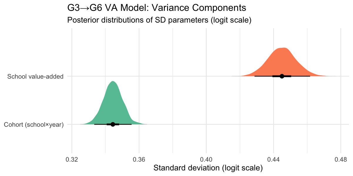
The latent-scale decomposition excludes the theoretical binomial observation variance (π²/3 ≈ 3.29). School VA and cohort noise together explain the remaining variation in G6 outcomes after conditioning on G3 quality, year×subject effects, and the binomial likelihood.
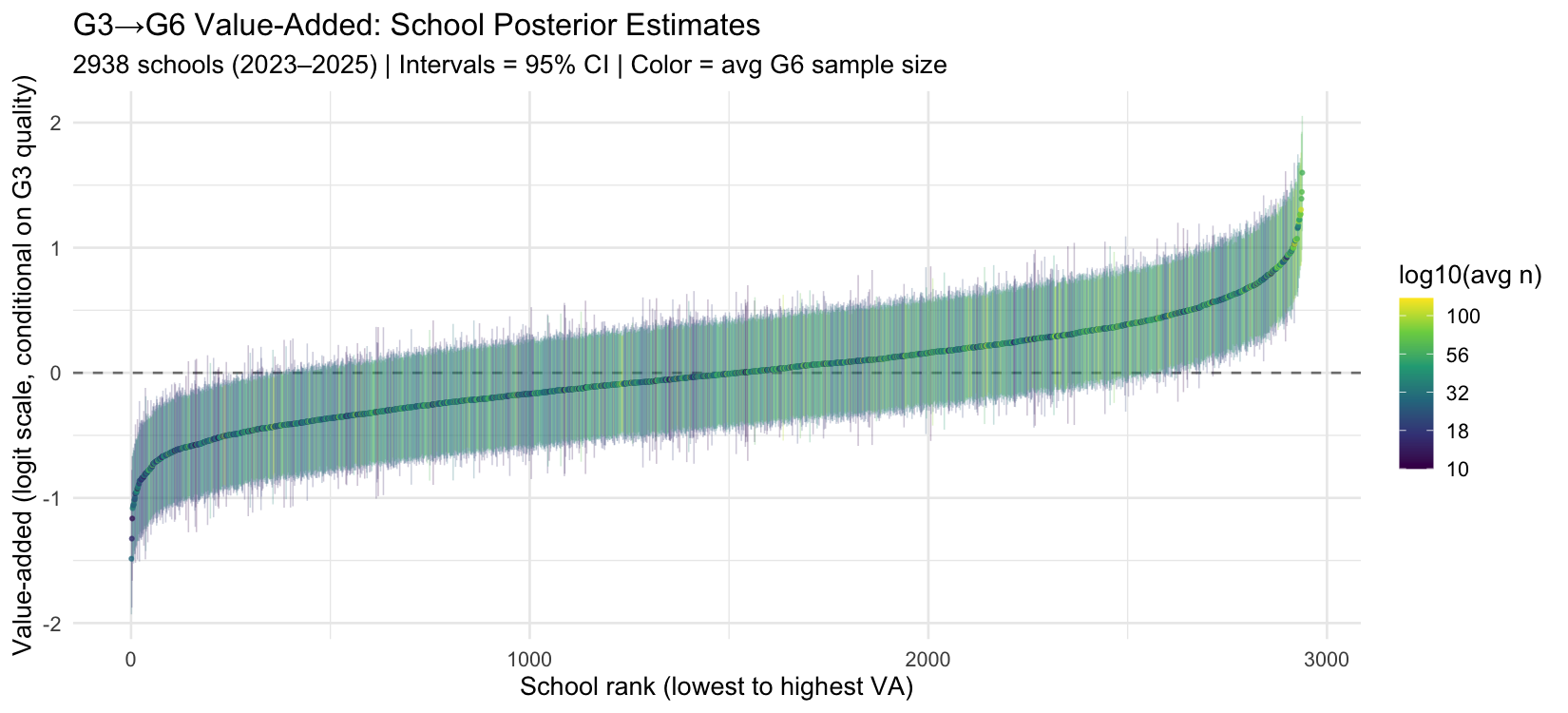
School value-added estimates
Ranked by posterior mean VA. Interval width reflects both sample size and how many years of G6 data the school has. Small-sample schools have wide intervals — the model is appropriately uncertain about labelling them high or low VA.
VA vs G3 quality scatter
This is the key diagnostic. If the G3 covariate failed to absorb intake-level differences, the VA estimates would be positively correlated with G3 quality (high-G3 schools would appear high-VA). A near-zero slope confirms the design is working.
Interpreting the residual correlation
The single-coefficient design uses one value for how G3 quality predicts G6 performance, averaged across all three subjects. But the G3→G6 trajectory is dramatically asymmetric by subject:
- Math: province-wide G3 ≈ 62%, G6 ≈ 50% — a ~12 pp drop as the curriculum shifts to fractions, algebra, and geometry.
- Reading and Writing: both increase substantially from G3 to G6 at the province level.
The year_subject fixed effects absorb these province-wide shifts. What they cannot absorb is whether the magnitude of the math drop varies with school quality. If high-G3 schools protect better against the G6 math difficulty spike — because good teaching matters more when the curriculum gets harder — their G6 VA will appear positive conditional on their G3 RE, producing r(VA, G3) > 0 even after proper conditioning.
The natural fix would be subject-specific G3 quality estimates in Stage 2 — three separate me() terms, each with its own coefficient. Given the near-flat G3 subject profiles those three covariates would be highly collinear (~0.85+ correlated across schools), so the gain is likely modest. The r = 0.216 is best read as honest residual uncertainty: some intake-level confounding remains, but it is not large enough to materially distort school VA rankings (rank-correlation across the old and new model versions: 0.97).
VA distribution by school size
Bayesian shrinkage means small schools have their VA pulled toward the prior mean (zero), while large schools are more influenced by their actual data. We should see: the spread of point estimates grows with school size (less shrinkage = more dispersed), while the 95% CI width shrinks (more data = tighter posterior).
Bayesian shrinkage: school size × G3 quality
When two schools produce identical observed G6 pass rates, their posterior (fitted) G6 results can diverge substantially — especially when their G3 quality differs and sample sizes are small.
The fitted G6 result is a weighted average of two poles:
fitted = (1 − λ) × [G3-quality-informed prior] + λ × [observed G6 data]
where λ = σ²_VA / (σ²_VA + σ²_obs/n) is the data-weight (Bayesian credibility factor). For small n, the prior dominates; for large n, the observed data dominates. A school with high G3 quality has a higher prior, so it gets "credited" for expected performance even when its observed results are average — and the smaller the school, the more that credit matters.
The chart below fixes raw observed G6 at the province average and varies n and G3 quality:
Residuals by G6 size and G3 quality
The VA estimates (school random effects) are the model residuals after conditioning on G3 quality. If the model is well-specified, these residuals should show no systematic trend against either school size or G3 quality.
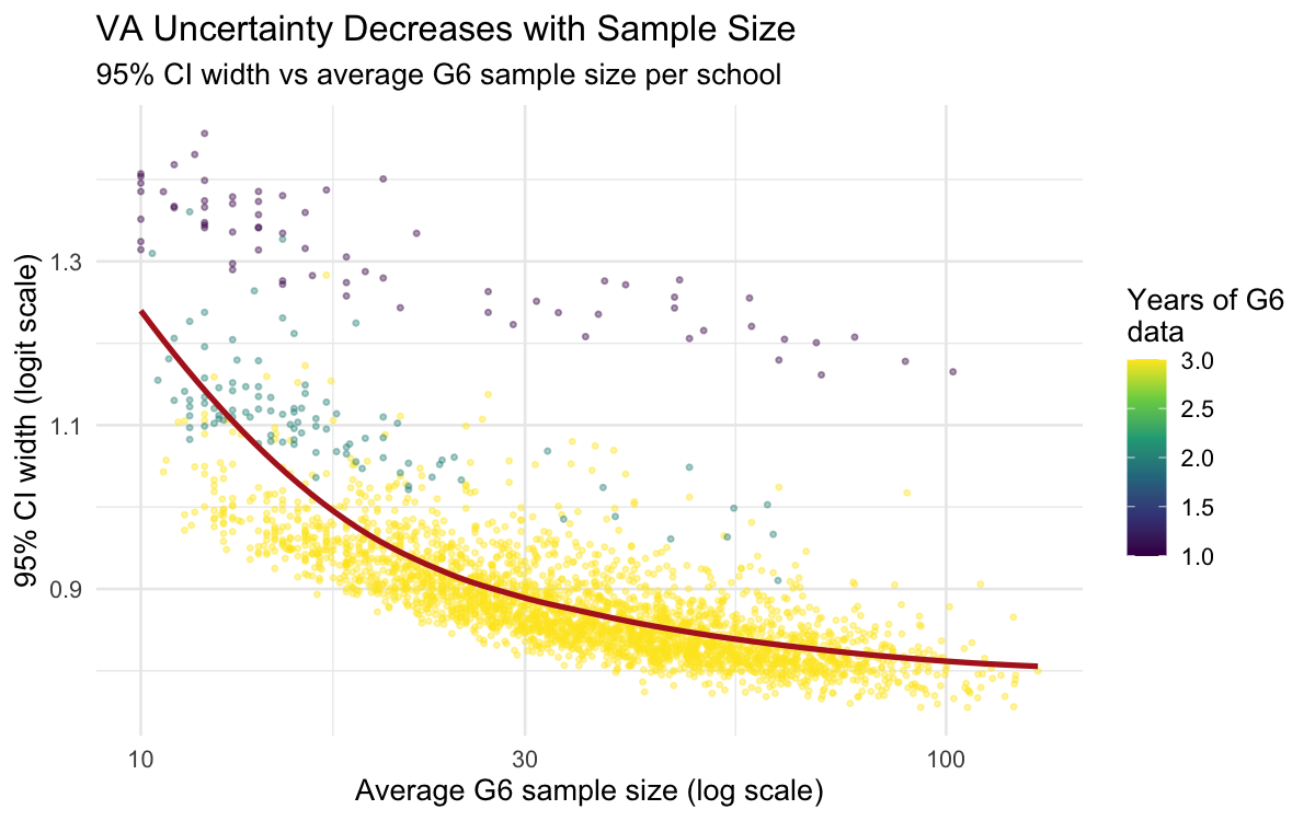
VA uncertainty vs sample size
Larger schools produce narrower credible intervals — the binomial likelihood automatically shrinks estimates more for small schools. This replaces the ad-hoc reliability formula (λ = σ²/(σ² + σ²ε/W)) from the frequentist model.
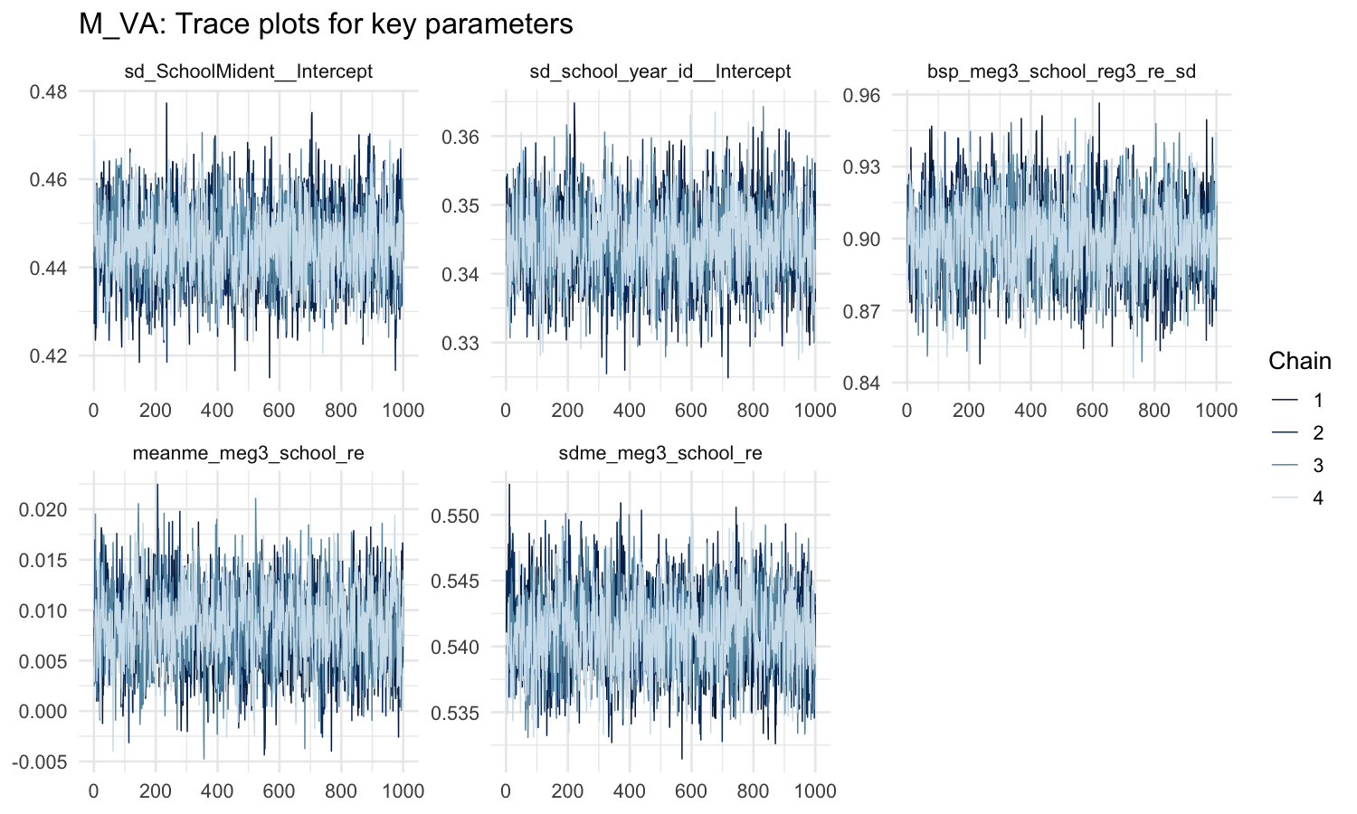
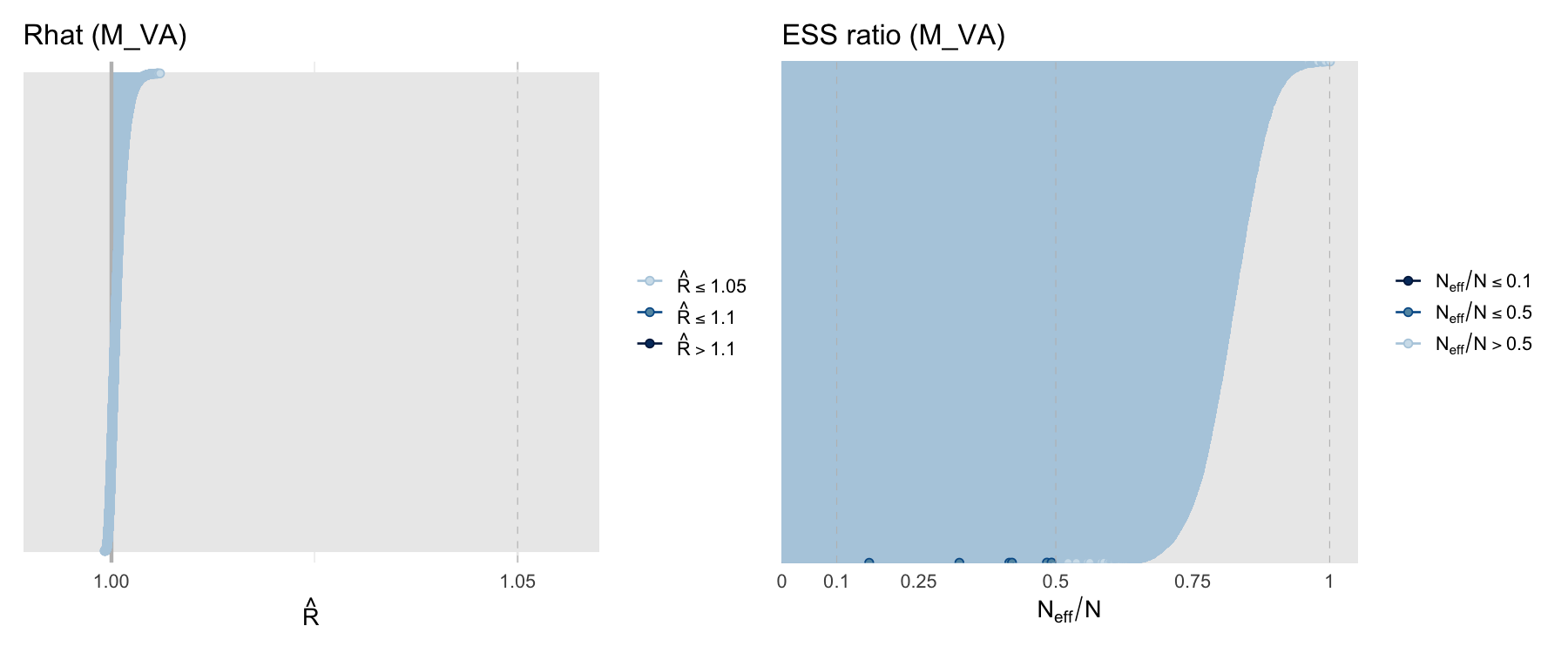
MCMC diagnostics
Comparison with frequentist approach
| Aspect | Frequentist (Python, logit-normal) | Bayesian (this page) |
|---|---|---|
| G3 signal | Single-year G3 scores per school | 3-year posterior G3 school RE |
| G6 likelihood | Logit-normal with manual weights | Exact binomial |
| Year coverage | 5 pair-types including 2022 | 2023–2025 only (avoids year quirks) |
| VA uncertainty | Ad-hoc reliability formula λ | 95% credible intervals directly |
| Confounding check | Mundlak correction (fixed effect) | G3 school RE as covariate |
| Subject-specific VA | Separate M_VA2 model | Extend with (1|school_subject_id) |