Bayesian Multilevel Model

A proper Bayesian binomial GLMM fitted with Stan via brms. Unlike the logit-normal approximation on the frequentist page, this model uses the exact binomial likelihood — sample size drives shrinkage automatically, with no ad-hoc weighting.

Method: Four models fitted progressively using brms (Bayesian regression models for Stan). M0: Normal on raw proportions (ignores sample size). M1: Binomial with school random intercepts (sample size matters). M2: + year×subject fixed effects + school×year cohort effects. M3: + school×subject profiles. Grade 3 English-language schools, 2022–23 through 2024–25 (3 years, 3 subjects). M0/M1 fitted on all 3,246 eligible schools; M2/M3 fitted on a 500-school stratified subsample for model comparison. A separate Stage 1 production fit (M2 on the full 3,246-school sample) is then used as input to the G3→G6 value-added model — see the section below.

Why the binomial likelihood matters

The single most important modelling choice: using y_success | trials(n_trials) instead of treating raw proportions as continuous.

A school that achieves 80% with 200 students is very different from one that achieves 80% with 15 students. The Normal model (M0) treats them identically — both shrink the same amount toward the grand mean. The Binomial model (M1) knows the first estimate is reliable and barely touches it, while aggressively shrinking the second.

M0: Normal (ignores sample size)

Every school shrinks equally toward the grand mean, regardless of how many students it has. The arrows (vertical lines from the diagonal) are uniform across the colour range.

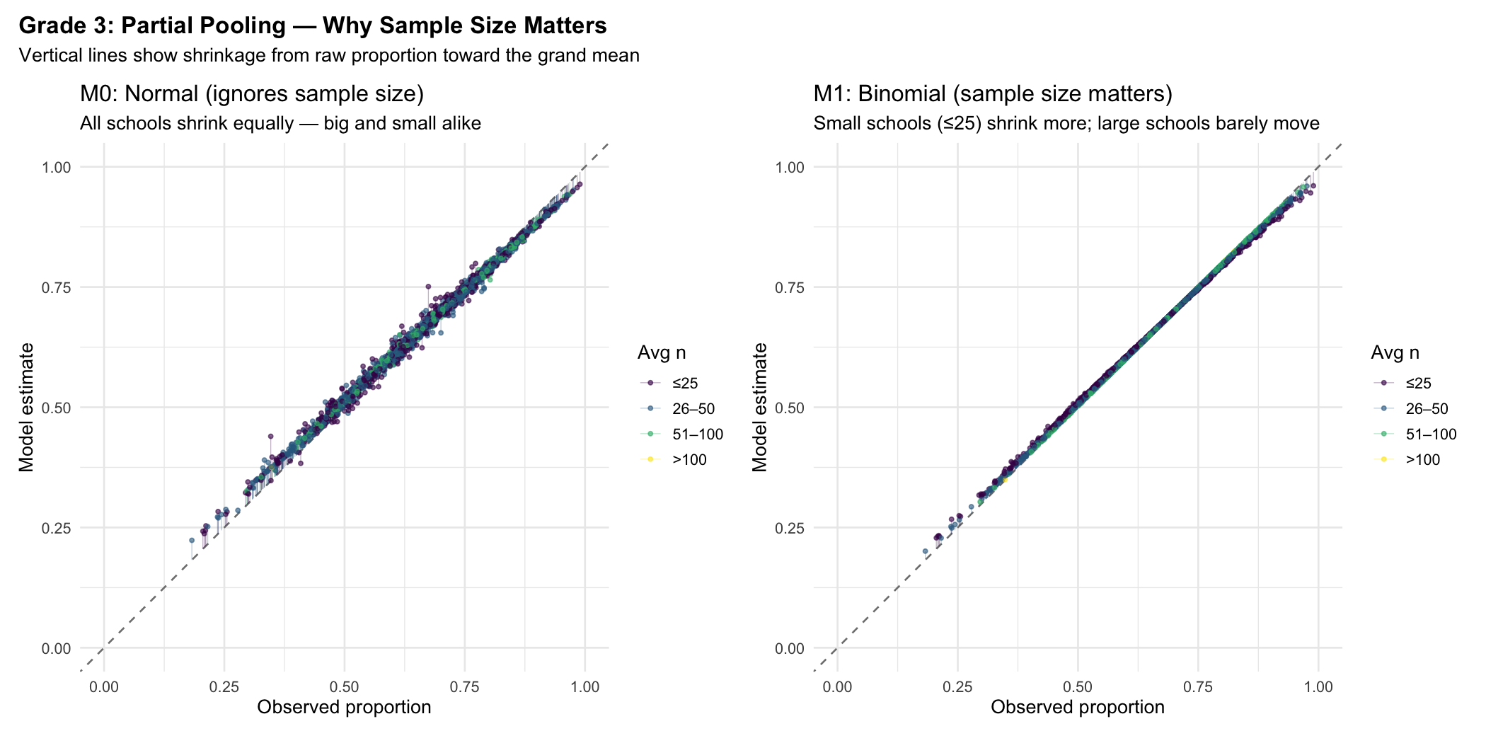
Shrinkage comparison: Normal vs Binomial

In the left panel, all schools get pulled toward the mean equally — the colour bands (sample size) don't matter. In the right panel, small schools (yellow, ≤25 students) are yanked hard toward the mean, while large schools (purple, >100) barely move. This is Gelman's partial pooling in action.

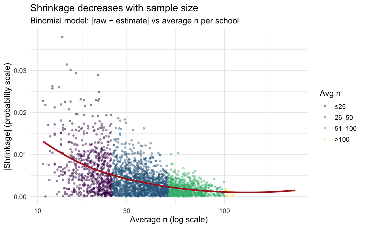
Shrinkage decreases with sample size

The relationship is monotone and dramatic. Schools with n > 100 barely shrink at all — their raw proportions are already reliable. Schools with n < 25 can move 10+ percentage points toward the grand mean.

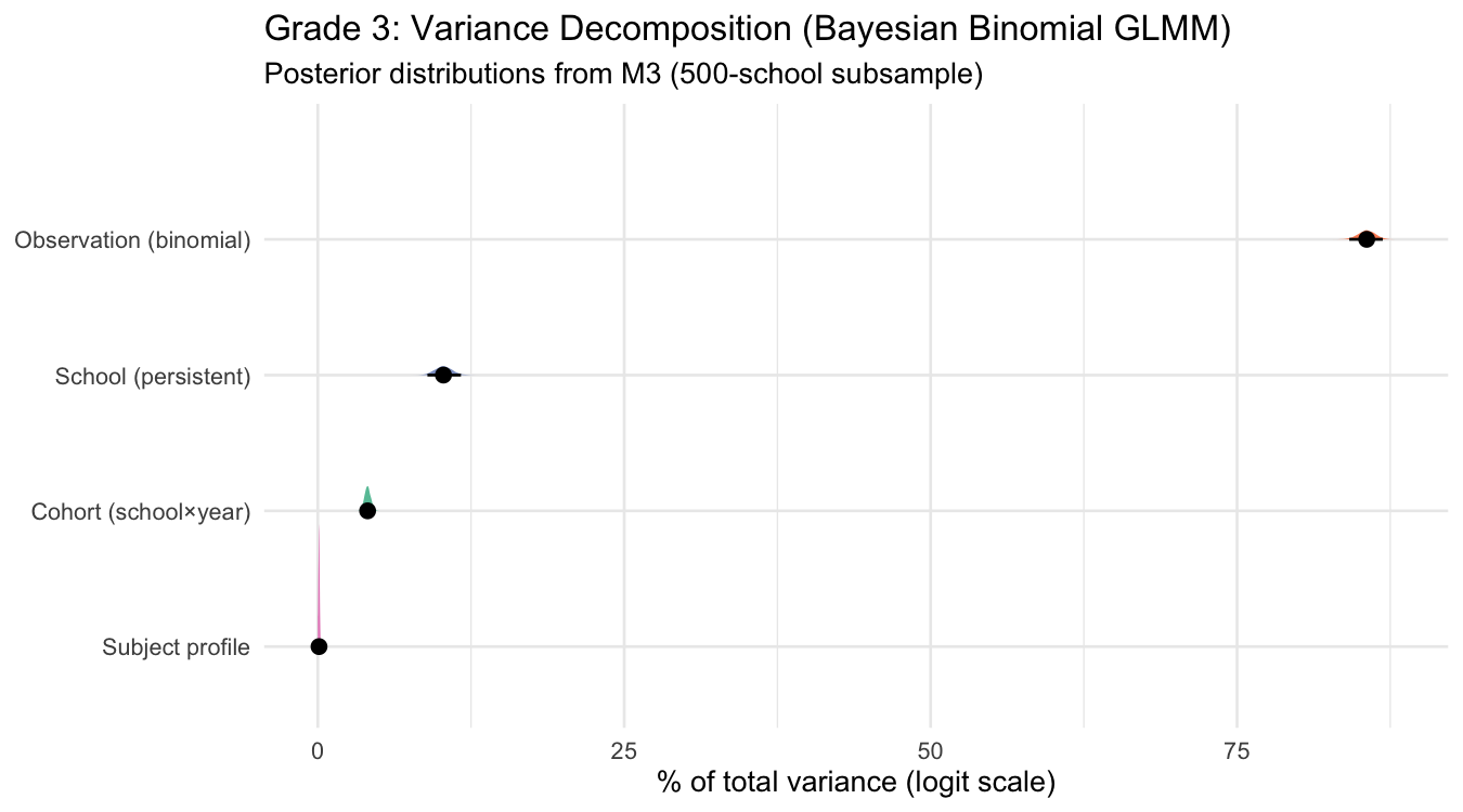
This is why ranking schools by raw L3/L4% is misleading for small schools. The Bayesian model gives better estimates by borrowing strength from the population. A small school that scores 95% isn't necessarily the best school — it might just be a school with 12 students where the binomial variance is enormous.

Variance decomposition

The full model (M3) decomposes variance in school×year×subject L3/L4 achievement into four sources. On the logit scale, the binomial observation-level variance (π²/3 ≈ 3.29) is a theoretical constant that dominates — so we show both the full decomposition and the latent-scale decomposition (excluding binomial noise).

Reading the halfeye plots: The thick bar is the 50% credible interval, the thin line is the 95% CI, and the dot is the posterior median. These are distributions, not point estimates — the full Bayesian posterior from 4,000 MCMC draws.

Full decomposition (logit scale, including binomial noise)

Component	Variance	% of total	Interpretation
Observation (binomial)	π²/3 = 3.29	85.6%	Binomial sampling noise (theoretical, not estimated)
School (persistent)	0.395 [0.339, 0.455]	10.3% [8.9%, 11.7%]	Stable school quality across years and subjects
Cohort (school×year)	0.156 [0.138, 0.177]	4.1% [3.6%, 4.6%]	Year-specific shared movement across subjects
Subject profile	0.004 [0.001, 0.008]	0.1% [0.0%, 0.2%]	School×subject divergence (e.g. strong in Math, weak in Writing)

Latent-scale decomposition (excluding binomial noise)

Removing the theoretical π²/3 term gives a view comparable to the frequentist logit-normal approximation:

Component	% of latent variance
School (persistent)	71.0% [66.7%, 75.0%]
Cohort (school×year)	28.2% [24.3%, 32.5%]
Subject profile	0.7% [0.1%, 1.4%]

The frequentist model on the main Multilevel Model page found: school ~57%, cohort ~21%, noise ~22%. The Bayesian model attributes more to persistent school quality and less to noise — partly because the binomial likelihood properly accounts for sampling variation that the logit-normal lumped into the residual.

Why is the subject profile so small? One might expect schools to vary meaningfully in subject emphasis — e.g. schools with many ELL students struggling more in reading, or a school with an exceptional math teacher outperforming in that subject. These effects are real, but they show up in other variance components rather than the subject profile:

Teacher quality is transient: An exceptional Grade 3 math teacher is there for a year or two, not permanently. That signal lands in the cohort (school×year) component, not the persistent subject profile.
ELL composition shifts all subjects: Schools with many English learners tend to score lower across reading, writing, and math — a level shift absorbed by the school intercept. A subject profile only emerges if ELL-heavy schools are systematically better at math relative to their own reading.
L3/L4% is a coarse threshold: Subject-specific strengths may appear in mean scores or level distributions but get masked by the binary "meeting standard" cut-off.
Grade 3 generalist teaching: Most G3 instruction comes from a single classroom teacher, limiting the scope for school-level subject specialization. The effect would likely be larger at G6 or G9.

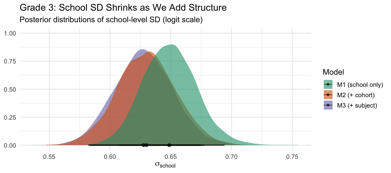
In short: schools probably do differ in subject emphasis, but those differences are mostly transient (captured by cohort effects) or masked by the outcome measure — not persistent enough across three years and three subjects to register as a large subject-profile variance.

School SD shrinks as we add structure

As we add random effects for cohorts and subject profiles, the school-level SD decreases. Some of what M1 attributed to "persistent school quality" was actually year-to-year cohort variation.

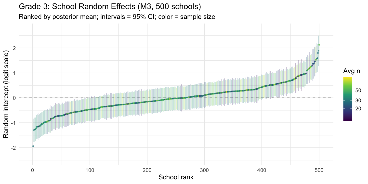
School random effects (caterpillar plot)

Each point is one school's posterior mean random intercept from M3, ranked from lowest to highest. The intervals are 95% credible intervals. Colour indicates average sample size — notice how small schools (yellow) have wider intervals.

Caterpillar plot of school random effects

Schools at the extremes have the widest uncertainty — the model is appropriately cautious about labelling a school as "best" or "worst" when the evidence is uncertain. The interval width is driven by both sample size (smaller n → wider) and distance from the mean (extreme values are more likely to be noise).

Model comparison (LOO-CV)

Leave-one-out cross-validation on the 500-school subsample confirms the progressive improvement:

Model	Description	ELPD diff	SE diff
M3	School + Cohort + Subject	0.0	—
M2	School + Cohort	−15.3	4.1
M1	School only	−2451.3	87.3

M3 (full model) wins decisively. The jump from M1 → M2 is massive (adding year×subject fixed effects and cohort random effects). The M2 → M3 improvement is smaller but significant (3.7 SE), confirming that subject profiles are a real — if modest — effect.

Stage 1 production model

The M0–M3 comparison above uses a 500-school subsample for speed. For the G3→G6 value-added pipeline, a separate Stage 1 production fit runs M2 on the full expanded sample:

Formula: y_success | trials(n_trials) ~ year_subject + (1 | school) + (1 | school_year_id)
Schools: 3,246 eligible G3 schools (expanded from ~2,646 by switching from a strict all-observations gate to observation-level filtering — individual observations with < 50% participation are dropped; schools need ≥ 2 observations at ≥ 70% participation)
School RE SD: 0.65 logit (posterior mean), Rhat ≈ 1.00 throughout
Output: g3_school_quality.parquet — one row per school with posterior mean (g3_school_re) and posterior SD (g3_re_sd) of the school random intercept

The posterior SD is carried into Stage 2 as a measurement-error input: me(g3_school_re, g3_re_sd). This corrects the attenuation bias from treating a noisy estimate as a fixed covariate — without it, the G3 coefficient is shrunk toward zero because the regressor contains estimation error. See the G3→G6 Value-Added page for Stage 2 details.

Why M2 (not M1) for Stage 1? M1 has only an intercept as a fixed effect, so year-to-year province-wide trends (curriculum changes, post-COVID recovery) bleed into school random intercepts. M2 absorbs these via year×subject fixed effects, producing a cleaner school quality signal as input to the VA model.

MCMC diagnostics

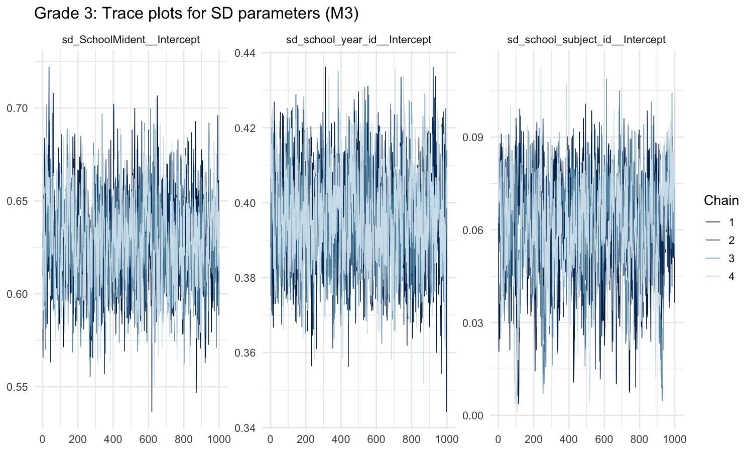
Trace plots

Well-mixed chains for the three SD hyperparameters. All four chains explore the same region of parameter space with no trends or sticky patches.

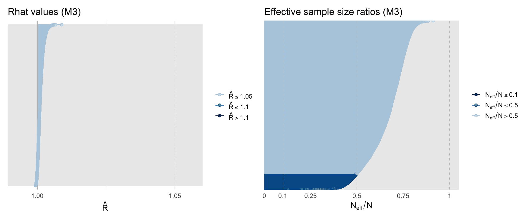
Convergence diagnostics

Rhat values near 1.00 indicate chains have converged. ESS ratio (effective sample size / total draws) above 0.1 indicates adequate mixing. Low ESS for individual school random effects is expected — 500 schools means 500+ parameters sharing 4,000 draws.

Comparison with frequentist approach

Aspect	Frequentist (statsmodels)	Bayesian (brms/Stan)
Likelihood	Logit-normal approximation	Exact binomial
Weights	Ad-hoc n·p·(1−p)	Built into likelihood
Uncertainty	Point estimates + SE	Full posterior distributions
Variance decomposition	By subtraction across models	Direct from joint posterior
Shrinkage	Implicit in BLUPs	Explicit, driven by n
Speed	Seconds	~20 minutes
Sample	All schools	M0/M1: all 3,246; M2/M3: 500 subsample; Stage 1 production M2: all 3,246

The two approaches broadly agree on the ranking of variance components (school >> cohort >> subject profile), but the Bayesian model is more principled about uncertainty and gives tighter school-level estimates by properly using the binomial likelihood.